Tutorial: Working with Mismatched INterface Theory (MINT) and the 3D MINT-Sandwich Approach
Betül Pamuk, ORCID 0000-0002-2817-0592
Drake Alexander Niedzielski, ORCID 0000-0002-9607-8042
Eli Gerber, ORCID 0000-0002-9594-6450
Eun-Ah Kim, ORCID 0000-0002-9554-4443
Tomás Alberto Arias, ORCID 0000-0001-5880-0260
DOI: 10.34863/seqm-4p70
The Materials-by-Design approach relies on strong theoretical capabilities to predict the properties of novel materials. Interface quantum materials are the focus of PARADIM’s in-house research and many of these materials have a lattice mismatch between the two materials at the interface.
Traditional ab initio techniques for calculating the electronic structure of materials are powerless when the lattice mismatch between two crystals leads to the absence of periodicity. The two common approaches to dealing with aperiodic systems are the cluster approach and the supercell approach. In the former case, one builds a large, isolated-cluster of the periodic material to simulate a mostly periodic structure. In the latter case, one builds a large periodic supercell of the aperiodic structure to enable the application of high performance techniques developed for periodic systems. Unfortunately, in both cases, the simulations become computationally expensive and time consuming as the simulation size increases. Both methods assume a convergence toward the exact behavior as the simulated material size reaches infinity. This assumption depends on the “nearsightedness” of electronic matter.
To overcome this issue, Prof. Kim and Prof. Arias have developed Mismatched Interface Theory (MINT) to study incommensurate interfaces. MINT combines the supercell and cluster approaches directly within standard density functional theory (DFT). The nearsightedness of the electronic matter also ensures that the convergences are achieved rather rapidly with MINT.
This tutorial provides an example of a MINT calculation for the incommensurate Graphene/α-RuCl3 interface. For further explanation of the theory behind MINT as well as converged results, please refer to E. Gerber et al. Phys. Rev. Lett. 124, 106804 (2020).
The calculations in the tutorial are performed by JDFTx (http://jdftx.org/) code, but the MINT theory is general enough that it can be used with the charge density output of any DFT code.
This tutorial assumes that the user is familiar with DFT. If the user is not familiar with DFT, we recommend looking into our PARADIM summer school videos, PARADIM tutorials (based on a different code, Quantum Espresso) as well as tutorials on the JDFTx website to familiarize yourself with how DFT calculations work.
Substrate Material, α-RuCl3
We first start with a large periodic supercell of the substrate material, which is the material system of primary interest, α-RuCl3 in this example.
lattice \
22.5252 0  0\
0    19.5068 0\
0     0     35

kpoint-folding 6 4 1
ion-species /home/bpamuk/scr4_tmcquee2/betul/MINT/MINT_tutorial_files_Eli/RUNS/pseudos/Ru_ONCV_PBE-1.0.upf
ion-species /home/bpamuk/scr4_tmcquee2/betul/MINT/MINT_tutorial_files_Eli/RUNS/pseudos/Cl_ONCV_PBE-1.0.upf
elec-cutoff 30

elec-n-bands 197  # num of valence e in u.c./2. 4*16+12*7+30=178/u.c.
elec-smearing Fermi 0.003
electronic-minimize energyDiffThreshold 0.00005

dump-name Ru8C14dens.$VAR
Dump End ElecDensity State
Dump End IonicPositions
Dump End Lattice

coords-type Cartesian

ion Ru  0       0       0       0
ion Ru  11.26262072     0       0       0
ion Ru  -0.009694315    6.425327665     -0.000321254    0
ion Ru  11.25292641     6.425327665     -0.000321254    0
ion Ru  -5.635911855    9.73609683      0.008352607     0
ion Ru  5.62670887      9.73609683      0.008352607     0
ion Ru  -5.634041022    16.27378784     -0.01273678     0
ion Ru  5.628579702     16.27378784     -0.01273678     0
ion Cl  -1.731672983    3.23689962      2.608280935     0
ion Cl  9.530947742     3.23689962      2.608280935     0
ion Cl  -1.955719372    16.4294827      2.545088364     0
ion Cl  9.306901353     16.4294827      2.545088364     0
ion Cl  -7.597187033    -0.130126808    2.566839156     0
ion Cl  3.665433692     -0.130126808    2.566839156     0
ion Cl  -7.587511615    6.635352257     2.568332043     0
ion Cl  3.675109109     6.635352257     2.568332043     0
ion Cl  -1.949880106    9.571803704     2.539456969     0
ion Cl  9.312740618     9.571803704     2.539456969     0
ion Cl  -7.323818691    13.01566655     2.54266951      0
ion Cl  3.938802034     13.01566655     2.54266951      0
ion Cl  -9.526922617    3.241359383     -2.602214902    0
ion Cl  -9.316482284    16.43628572     -2.551229987    0
ion Cl  -3.657893669    -0.125402483    -2.569919416    0
ion Cl  1.735698108     3.241359383     -2.602214902    0
ion Cl  1.946157338     16.43628572     -2.551229987    0
ion Cl  7.604727055     -0.125402483    -2.569919416    0
ion Cl  -3.653868544    6.631308235     -2.549510332    0
ion Cl  1.940488148     9.560559811     -2.535242871    0
ion Cl  7.60875218      6.631308235     -2.549510332    0
ion Cl  -9.322132577    9.560559811     -2.535242871    0
ion Cl  -3.94106971     13.00948714     -2.54805524     0
ion Cl  7.321551015     13.00948714     -2.54805524     0

spintype z-spin
initial-magnetic-moments Ru 1 -1 -1 1 1 -1 -1 1 Cl 0 0 0 0 0 0 0 0 0 0 0 0 0 0 0 0 0 0 0 0 0 0 0 0
Cluster Material, Graphene Flake
Next, we create a cluster, a graphene flake in this example, such that the adjacent cluster images do not interact with each other. (Note that, in this example, we also terminate the edges of the flake with hydrogen atoms to eliminate dangling bonds and increase the rate of convergence with flake size.) Here is an example of a flake with 14 C sites:
lattice \
22.5252 0  0\
0    19.5068 0\
0     0     35
kpoint-folding 6 4 1
ion-species /home/bpamuk/scr4_tmcquee2/betul/MINT/MINT_tutorial_files_Eli/RUNS/pseudos/C_ONCV_PBE-1.0.upf
ion-species /home/bpamuk/scr4_tmcquee2/betul/MINT/MINT_tutorial_files_Eli/RUNS/pseudos/H_ONCV_PBE-1.0.upf

elec-cutoff 30

elec-n-bands 197  # num of valence e in u.c./2. 4*16+12*7+30=178/u.c.
elec-smearing Fermi 0.003

electronic-minimize energyDiffThreshold 0.00005

dump-name Ru8C14dens.$VAR
Dump End ElecDensity State
Dump End IonicPositions
Dump End Lattice
coords-type Cartesian
ion C   4.67050549      8.653759177     6.584456559867589       0
ion C   6.893392999     7.345691851     6.584456559867589       0
ion C   6.893392999     4.654308149     6.584456559867589       0
ion C   4.67050549      3.346240823     6.584456559867589       0
ion C   -4.67050549     3.346240823     6.584456559867589       0
ion C   -6.893392999    4.654308149     6.584456559867589       0
ion C   -6.893392999    7.345691851     6.584456559867589       0
ion C   -4.67050549     8.653759177     6.584456559867589       0
ion C   0       8.648964932     6.584456559867589       0
ion C   0       3.351035068     6.584456559867589       0
ion C   2.302773955     7.361204644     6.584456559867589       0
ion C   2.302773955     4.638795356     6.584456559867589       0
ion C   -2.302773955    4.638795356     6.584456559867589       0
ion C   -2.302773955    7.361204644     6.584456559867589       0
ion H   4.659683006     10.702098       6.584456559867589       0
ion H   8.678469751     8.345243747     6.584456559867589       0
ion H   8.678469751     3.654756253     6.584456559867589       0
ion H   4.659683006     1.297902004     6.584456559867589       0
ion H   -4.659683006    1.297902004     6.584456559867589       0
ion H   -8.678469751    3.654756253     6.584456559867589       0
ion H   -8.678469751    8.345243747     6.584456559867589       0
ion H   -4.659683006    10.702098       6.584456559867589       0
ion H   0       10.69934088     6.584456559867589       0
ion H   0       1.30065912      6.584456559867589       0

spintype z-spin
initial-magnetic-moments C 1 -1 1 -1 1 -1 1 -1 1 -1 1 -1 1 -1 H 0 0 0 0 0 0 0 0 0 0
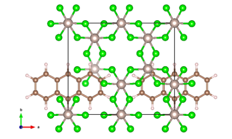
MINT bilayer interface, Graphene/α-RuCl3
Next, we place the graphene flake on top of the substrate α-RuCl3 and relax the ionic coordinates:
lattice \
22.5252 0  0\
0    19.5068 0\
0     0     35

kpoint-folding 6 4 1

ion-species /home/bpamuk/scr4_tmcquee2/betul/MINT/MINT_tutorial_files_Eli/RUNS/pseudos/Ru_ONCV_PBE-1.0.upf
ion-species /home/bpamuk/scr4_tmcquee2/betul/MINT/MINT_tutorial_files_Eli/RUNS/pseudos/Cl_ONCV_PBE-1.0.upf
ion-species /home/bpamuk/scr4_tmcquee2/betul/MINT/MINT_tutorial_files_Eli/RUNS/pseudos/C_ONCV_PBE-1.0.upf
ion-species /home/bpamuk/scr4_tmcquee2/betul/MINT/MINT_tutorial_files_Eli/RUNS/pseudos/H_ONCV_PBE-1.0.upf

elec-cutoff 30

elec-n-bands 197  # num of valence e in u.c./2. 4*16+12*7+30=178/u.c.
elec-smearing Fermi 0.003
#lattice-minimize energyDiffThreshold 0.0001 nIterations 10
#ionic-minimize energyDiffTHreshold 0.0001 nIterations 10
electronic-minimize energyDiffThreshold 0.00005

dump-name Ru8C14dens.$VAR
Dump End ElecDensity State
Dump End IonicPositions
Dump End Lattice
coords-type Cartesian
ion C   4.67050549      8.653759177     6.584456559867589       0
ion C   6.893392999     7.345691851     6.584456559867589       0
ion C   6.893392999     4.654308149     6.584456559867589       0
ion C   4.67050549      3.346240823     6.584456559867589       0
ion C   -4.67050549     3.346240823     6.584456559867589       0
ion C   -6.893392999    4.654308149     6.584456559867589       0
ion C   -6.893392999    7.345691851     6.584456559867589       0
ion C   -4.67050549     8.653759177     6.584456559867589       0
ion C   0       8.648964932     6.584456559867589       0
ion C   0       3.351035068     6.584456559867589       0
ion C   2.302773955     7.361204644     6.584456559867589       0
ion C   2.302773955     4.638795356     6.584456559867589       0
ion C   -2.302773955    4.638795356     6.584456559867589       0
ion C   -2.302773955    7.361204644     6.584456559867589       0
ion H   4.659683006     10.702098       6.584456559867589       0
ion H   8.678469751     8.345243747     6.584456559867589       0
ion H   8.678469751     3.654756253     6.584456559867589       0
ion H   4.659683006     1.297902004     6.584456559867589       0
ion H   -4.659683006    1.297902004     6.584456559867589       0
ion H   -8.678469751    3.654756253     6.584456559867589       0
ion H   -8.678469751    8.345243747     6.584456559867589       0
ion H   -4.659683006    10.702098       6.584456559867589       0
ion H   0       10.69934088     6.584456559867589       0
ion H   0       1.30065912      6.584456559867589       0
ion Ru  0       0       0       0
ion Ru  11.26262072     0       0       0
ion Ru  -0.009694315    6.425327665     -0.000321254    0
ion Ru  11.25292641     6.425327665     -0.000321254    0
ion Ru  -5.635911855    9.73609683      0.008352607     0
ion Ru  5.62670887      9.73609683      0.008352607     0
ion Ru  -5.634041022    16.27378784     -0.01273678     0
ion Ru  5.628579702     16.27378784     -0.01273678     0
ion Cl  -1.731672983    3.23689962      2.608280935     0
ion Cl  9.530947742     3.23689962      2.608280935     0
ion Cl  -1.955719372    16.4294827      2.545088364     0
ion Cl  9.306901353     16.4294827      2.545088364     0
ion Cl  -7.597187033    -0.130126808    2.566839156     0
ion Cl  3.665433692     -0.130126808    2.566839156     0
ion Cl  -7.587511615    6.635352257     2.568332043     0
ion Cl  3.675109109     6.635352257     2.568332043     0
ion Cl  -1.949880106    9.571803704     2.539456969     0
ion Cl  9.312740618     9.571803704     2.539456969     0
ion Cl  -7.323818691    13.01566655     2.54266951      0
ion Cl  3.938802034     13.01566655     2.54266951      0
ion Cl  -9.526922617    3.241359383     -2.602214902    0
ion Cl  -9.316482284    16.43628572     -2.551229987    0
ion Cl  -3.657893669    -0.125402483    -2.569919416    0
ion Cl  1.735698108     3.241359383     -2.602214902    0
ion Cl  1.946157338     16.43628572     -2.551229987    0
ion Cl  7.604727055     -0.125402483    -2.569919416    0
ion Cl  -3.653868544    6.631308235     -2.549510332    0
ion Cl  1.940488148     9.560559811     -2.535242871    0
ion Cl  7.60875218      6.631308235     -2.549510332    0
ion Cl  -9.322132577    9.560559811     -2.535242871    0
ion Cl  -3.94106971     13.00948714     -2.54805524     0
ion Cl  7.321551015     13.00948714     -2.54805524     0

spintype z-spin
initial-magnetic-moments Ru 1 -1 -1 1 1 -1 -1 1 Cl 0 0 0 0 0 0 0 0 0 0 0 0 0 0 0 0 0 0 0 0 0 0 0 0 C 1 -1 1 -1 1 -1 1 -1 1 -1 1 -1 1 -1 H 0 0 0 0 0 0 0 0 0 0
Once we obtain the optimized ionic positions of the interface, we calculate the charge density of each component of the MINT calculation, i.e., the substrate, the flake, and the interface, separately.
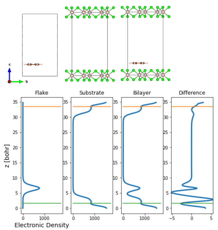
Once the electronic density is obtained, one can plot the variation of the electronic charge density along the z-axis as shown above. The integral of the charge density yields the charge transfer between the substrate and the flake. At this point, the user needs to determine up to which the z-coordinate the charge transfer occurs — we suggest this to be taken to be the point where there is a minima in the charge density plots, as indicated by the green and orange lines above.
After the integration of the charge density up to the green line, we obtain the charge transfer to the α-RuCl3 layer to be 0.0096 e-/C atom. We then scale this value to the transfer expected for a full graphene layer L by multiplying by N(L)/N(C), the ratio of the (incommensurate) number of carbon atoms expected for a full graphene layer N(L) and the number in each cluster N(C), which is N(L)/N(C)=5.7. Therefore, for this particular example of 14 C-site graphene flake, the charge transfer is about 5.472% which is a value comparable to that obtained in the referenced manuscript.
Shifting the flake position:
Next, to further improve convergence with flake size, it is useful to repeat the above step, shifting the flake position on the substrate along the x-y plane, relaxing the ionic positions for each shifted flake, and finally taking the average of the charge transfer from several different flake positions. This allows for sampling all possible registries between the two monolayers, which is particularly important for small flake sizes. We leave this step to the user.
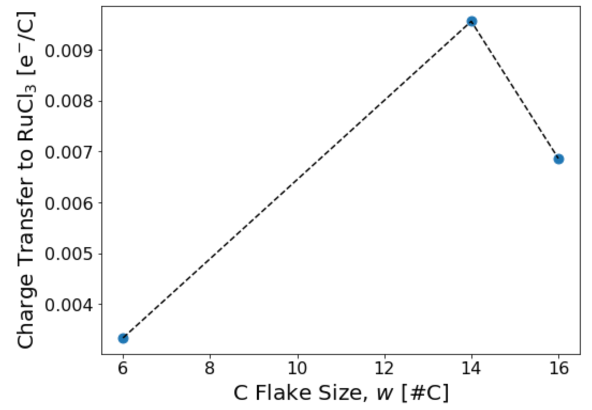
Change the flake size:
Finally, we vary the flake size to obtain the asymptotic limit of infinite flake size. For demonstration purposes, here we plot results for graphene flakes with 6 C atoms, 14 C atoms, and 16 C atoms. One can see that the charge transfer increases as the flake size increases initially. The fluctuation in the charge transfer as one goes from 14 to 16 C atom sites shows the importance of shifting the flake position on the substrate and taking an average of the charge transfer.
Once the charge transfer is sampled properly for each flake size and this calculation is repeated for several increasing flake sizes, one should get the result presented in the paper: E. Gerber et al. Phys. Rev. Lett. 124, 106804 (2020).
Nearsightedness of electronic matter ensures that, sufficiently far from the boundary of the flake, both materials behave just as they would for a truly infinite interface. Moreover, as the flake size increases, it eventually samples all possible registries with the other material. Appropriate finite-size scaling of thermodynamically intrinsic quantities then enables extraction of the behavior of the infinite interface.
Below we present a python script in text format which in the future will also be hosted on our website as a Jupyter notebook. This script directly generates Fig. 3 of this tutorial.
# Electron density reading code adapted from JDFTx tutorial
# https://jdftx.org/Outputs.html
import numpy as np
import re
import matplotlib.pyplot as plt

# The user sets the following variables
#############################################################################
MINTpath = "../RUNS"  # Folder that contains the flakeDirs
nSubsLayers = 1                         # Number of substrate layers
flakeSizes = [6,14,16]                  # Number of atoms of interest (e.g. C for Graphene/RuCl3) per flake
flakeDirs = ["/6Site","/14Site","/16Site"] # Names of dirs in MINTpath, must match length of flakeSizes
shiftDirs = ["/shift000"] #,"/shift025","/shift050","/shift075"] # sub dirs for different flake displacement/orientations
# Make sure that shiftDirs is the union of the set of sub dir names over all flakeDirs

# Mark True if your spin up and spin down electron densities are split into two separate files
#    Also make sure to edit "nfile_up" and "nfile_dn"
spinPolar = True #False

outfile = "/totalE.out"       # All .out files must have this name
nfile = "/system.n"           # All .n files must have this name
nfile_up = "/system.n_up"     # All .n_up files must have this name (only need if spinPolar = True)
nfile_dn = "/system.n_dn"     # All .n_dn files must have this name (only need if spinPolar = True)
latfile = "/system.lattice"   # All .lattice files must have this name
ionposfile = "/system.ionpos" # All .ionpos files must have this name
# each MINTpath/flakeDir/shiftDir has these 3 folders for the full bilayer, isolated flake, and isolated substrate
#
BL_dir = "/bilayer"               # /directory for the interface
Flake_dir = "/isolated_flake"     # /directory for the isolated flake
Subs_dir = "/isolated_substrate"  # /directory for the isolated substrate

# Interface cutoff ranges:
# You will almost certainly have to change these for your system
# The interface btw the flake and the substrate is defined as the place where the total
#   electron density takes a minimum btw the two layers
# These four variables determine the bounds where the code will look for those interfaces
# units = fraction of unit cell height
lowerInterfaceBotGuess = 0.00
lowerInterfaceTopGuess = 0.05
upperInterfaceBotGuess = 0.95
upperInterfaceTopGuess = 1.00

# Plotting Labels
R_name = 'C'           # Name of the atomic species you report charge transfer in (e.g. R_name='C' -> dQ = 0.1 e-/C)
Subs_name = 'RuCl$_3$' # Name of the periodic substrate material
Flake_name = 'C'       # Name of the flake material

# Plots: Axis Label, Tick Font Size, Figure Size
fs = 20
fs_tick = 16
figsize = (8*0.8,6*0.8)
############################################################################

# Total electron density files
outfilename_tot = BL_dir+outfile         #'/Bilayer/totalE.out'
densityfilename_tot = BL_dir+nfile             #'/Bilayer/totalE.n'
densityfilename_tot_up = BL_dir+nfile_up       #'/Bilayer/totalE.n'
densityfilename_tot_dn = BL_dir+nfile_dn       #'/Bilayer/totalE.n'
# Flake Electron Density files
outfilename_flake = Flake_dir+outfile    #'/isolated_flake/totalE.out'
densityfilename_flake = Flake_dir+nfile        #'/isolated_flake/totalE.n'
densityfilename_flake_up = Flake_dir+nfile_up  #'/isolated_flake/totalE.n'
densityfilename_flake_dn = Flake_dir+nfile_dn  #'/isolated_flake/totalE.n'
# Substrate Electron Density files
outfilename_subs = Subs_dir+outfile      #'/isolated_substrate/totalE.out'
densityfilename_subs = Subs_dir+nfile          #'/isolated_substrate/totalE.n'
densityfilename_subs_up = Subs_dir+nfile_up    #'/isolated_substrate/totalE.n'
densityfilename_subs_dn = Subs_dir+nfile_dn    #'/isolated_substrate/totalE.n'

# return a list of all lines in filename with pattern
def grep(pattern, filename):
    retval = []
    foundPattern = False
    file = open(filename, "r")
    for line in file:
        if re.search(pattern, line):
            retval.append(line)
            foundPattern = True
    if not foundPattern:
        print("grep failed to find:", pattern, "in", filename)
        print("returning an empty list")
    return retval

def finalFreeEnergy(filename):
    return float(grep("F =",filename)[0].split()[2])

def get_ionpos_ionsp(path2file):
    ionspecies = []
    ionpos = []
    with open(path2file,'r') as file:
        # Skip the comment line at the top of the file
        line = file.readline()
        # record ionspecies, and lattice coordinate
        while line:
            line = file.readline()
            line_text = line.split()
            if len(line_text) > 0:
                if line_text[0] == "ion":
                    ionspecies.append(line_text[1])
                    ionpos.append([float(x) for x in line_text[2:5]])
    return ionpos,ionspecies

def get_LatticeMatrix(path2file):
    LatticeMatrix = []
    with open(path2file,'r') as file:
        # skip the first two lines
        #line = file.readline()
        line = file.readline()
        # get the contents as a list of lines
        contents = file.readlines()
        LM = [line.split()[:3] for line in contents]
        LatticeMatrix = np.array([ [float(i) for i in lm] for lm in LM ])
    return LatticeMatrix

# Looks for the minima in the Bilayer Electron density
# to determine where the RS flake ends and the TMD substrate begins
# z_min and z_max are initial guesses
def get_flake_range(n_BL,a,b,c,d):
    z_bot = n_BL.index(min(n_BL[a:b]))
    z_top = n_BL.index(min(n_BL[c:d]))
    return z_bot,z_top

# returns the total electron transfer onto the flake
def get_tot_dQ(diff,flake_bot,flake_top,dV):
    # Sum together the charge transfer from the average value bins
    tot_dQ = np.sum(diff[flake_bot:flake_top]) * dV
    #print("tot_dQ_naive =",tot_dQ)
    return tot_dQ

def get_CT(path,nSubsLayers,debug=False):
    LM = get_LatticeMatrix(path+BL_dir+latfile)
    ionpos,ionsp = get_ionpos_ionsp(path+BL_dir+ionposfile)
    a,b,c = LM.T
    cs = np.cross(a,b)/np.linalg.norm(np.cross(a,b)) # orthogonal to a and b
    Lz = np.dot(c,cs)  # bohr , for plotting purposes
    ionpos = np.matmul(ionpos,np.transpose(LM))
    NR = ionsp.count(str(ionsp[0]))
    NT = ionsp.count(str(ionsp[NR]))
    Y1z = float(np.dot(ionpos[NR+NT  ],cs)) % Lz
    Y2z = float(np.dot(ionpos[NR+NT+1],cs)) % Lz
    R1z = float(np.dot(ionpos[0],cs)) % Lz
    R2z = float(np.dot(ionpos[1],cs)) % Lz
    X1z = float(np.dot(ionpos[-1],cs)) % Lz
    X2z = float(np.dot(ionpos[-2],cs)) % Lz
    atomPlanes = [0.0,Y1z,R1z,X1z,X2z,R2z,Y2z]

    if spinPolar:
        n_tot_up = np.fromfile(path+densityfilename_tot_up,   # read from binary file
                  dtype=np.float64)      # as 64-bit (double-precision) floats
        #n = swapbytes(n)                # uncomment on big-endian machines; data is always stored litte-endian
        n_tot_dn = np.fromfile(path+densityfilename_tot_dn,   # read from binary file
                  dtype=np.float64)      # as 64-bit (double-precision) floats
        #n = swapbytes(n)                # uncomment on big-endian machines; data is always stored litte-endian
        n_tot = n_tot_up + n_tot_dn

        n_flake_up = np.fromfile(path+densityfilename_flake_up,   # read from binary file
                  dtype=np.float64)      # as 64-bit (double-precision) floats
        #n = swapbytes(n)                # uncomment on big-endian machines; data is always stored litte-endian
        n_flake_dn = np.fromfile(path+densityfilename_flake_dn,   # read from binary file
                  dtype=np.float64)      # as 64-bit (double-precision) floats
        #n = swapbytes(n)                # uncomment on big-endian machines; data is always stored litte-endian
        n_flake = n_flake_up + n_flake_dn

        n_subs_up = np.fromfile(path+densityfilename_subs_up,   # read from binary file
                  dtype=np.float64)      # as 64-bit (double-precision) floats
        #n = swapbytes(n)                # uncomment on big-endian machines; data is always stored litte-endian
        n_subs_dn = np.fromfile(path+densityfilename_subs_dn,   # read from binary file
                  dtype=np.float64)      # as 64-bit (double-precision) floats
        #n = swapbytes(n)                # uncomment on big-endian machines; data is always stored litte-endian
        n_subs = n_subs_up + n_subs_dn
    else:
        n_tot = np.fromfile(path+densityfilename_tot,   # read from binary file
                  dtype=np.float64)      # as 64-bit (double-precision) floats
        #n = swapbytes(n)                # uncomment on big-endian machines; data is always stored litte-endian
        n_flake = np.fromfile(path+densityfilename_flake,   # read from binary file
                  dtype=np.float64)      # as 64-bit (double-precision) floats
        #n = swapbytes(n)                # uncomment on big-endian machines; data is always stored litte-endian

        n_subs = np.fromfile(path+densityfilename_subs,   # read from binary file
                  dtype=np.float64)      # as 64-bit (double-precision) floats
    #n = swapbytes(n)                # uncomment on big-endian machines; data is always stored litte-endian
    ns = [n_tot,n_flake,n_subs]
    ofs = [outfilename_tot,outfilename_flake,outfilename_subs]

    n = n_tot
    outfilename = outfilename_tot
    #look for the first instance of the following in the output file
    #unit cell volume =
    #Chosen fftbox size, =
    S = []
    V = 0
    flag = 0
    with open(path+outfilename,'r') as file:
        line = file.readline()
        #print(line)
        while line:
            line = file.readline()
            contents = line.split()
            #
            if len(contents) > 0:
                if contents[0] == "unit":
                    V = float(contents[4])
                    flag += 1
                elif contents[0] == "Chosen":
                    S = [int(contents[6]),int(contents[7]),int(contents[8])]
                    flag += 1

            if flag >= 2:
                break
    dV = V / np.prod(S)

    # Total Bilayer electron density
    n_tot_slices = []
    for z in range(S[2]):
        nz = n_tot.reshape(S)[:,:,z]
        # Sum up the electron density
        # choose a xy slice slice of the electron density
        slicedensity = np.sum(nz)
        # add it to an array for plotting
        n_tot_slices.append(slicedensity)

    # Sum of isolated_flake and isolated_substrate electron densities
    n_flake_slices = []
    n_subs_slices = []
    n_sum_slices = []
    for z in range(S[2]):
        nz_flake = n_flake.reshape(S)[:,:,z]
        nz_subs  = n_subs.reshape(S)[:,:,z]
        # Sum up the electron density
        # choose a xy slice slice of the electron density
        density_flake = np.sum(nz_flake)
        density_subs = np.sum(nz_subs)
        # add it to an array for plotting
        n_flake_slices.append(density_flake)
        n_subs_slices.append(density_subs)
        n_sum_slices.append(density_flake+density_subs)

    # Average charge difference as a function of z
    diff = [n_tot_slices[i]-n_sum_slices[i] for i in range(S[2])]

    # Interface cutoffs are the minima of the total electron density in
    #  the ranges specified by the user
    a = int(lowerInterfaceBotGuess * len(n_tot_slices))
    b = int(lowerInterfaceTopGuess * len(n_tot_slices))
    c = int(upperInterfaceBotGuess * len(n_tot_slices))
    d = int(upperInterfaceTopGuess * len(n_tot_slices))
    flake_bot,flake_top = get_flake_range(n_tot_slices,a,b,c,d)

    if debug:
        zbot = flake_bot*Lz/S[2]
        ztop = flake_top*Lz/S[2]
        z_plot = np.arange(0,Lz,Lz/S[2])

        fig, axes = plt.subplots(nrows=1, ncols=4, figsize=(8, 5))
        titles = ["Flake","Substrate","Bilayer","Difference"]
        n_data = [n_flake_slices,n_subs_slices,n_tot_slices,diff]
        axes[0].set_xlabel("Electronic Density",fontsize=14)
        axes[0].set_ylabel("z [bohr]",fontsize=14)
        axes[3].set_xlim([np.min(diff), np.max(diff)])
        for i in range(4):
            axes[i].plot(n_data[i],z_plot,linewidth=3)
            axes[i].set_title(titles[i])
            axes[i].plot((-5,1750),(ztop,ztop))
            axes[i].plot((-5,1750),(zbot,zbot))
        #fig.tight_layout()
        plt.show()

    # Sum up the charge difference on the flake
    return get_tot_dQ(diff,flake_bot,flake_top,dV)

def get_BE(path):
    E_bl  = finalFreeEnergy(path+BL_dir+outfile)
    E_rs  = finalFreeEnergy(path+Flake_dir+outfile)
    E_tmd = finalFreeEnergy(path+Subs_dir+outfile)
    return E_bl - (E_rs + E_tmd)

print("""Use the plots below to tune lowerInterfaceBotGuess, lowerInterfaceTopGuess,
         upperInterfaceBotGuess, and upperInterfaceTopGuess""")
print("Green Line  = Lower Material Interface")
print("Organe Line = Upper Material Interface")

flag = True # for plotting one debug plot
CTs = [] # Charge Transfers
BEs = [] # Binding Energies
for flakeDir in flakeDirs:
    CTs_flake = []
    BEs_flake = []
    for shiftDir in shiftDirs:
        path = MINTpath+flakeDir+shiftDir
        # Not all flake dirs have all the shiftDirs, account for this
        try:
            CT = get_CT(path,nSubsLayers,debug=flag)
            CTs_flake.append(CT)
            BE = get_BE(path)
            BEs_flake.append(BE)
        except:
            print("Warning: Couldn't compute either CT or BE in", path)
        if flag:
            flag = False
    CTs.append(CTs_flake)
    BEs.append(BEs_flake)

print("")
print("Raw Charge Transfers:")
print(CTs)

# Plot wrt inverse flake size and fit line to the converging datapoints
# The converged charge transfer will be the y-intercept
inv_flakeSizes = 1.0/np.array(flakeSizes)

# Plot the charge transfer v.s. Flake Size
CT_perR = [ [-1*np.array(CTs[i])/flakeSizes[i]] for i in range(len(flakeSizes))]
avgCT_perR = [np.mean(ctf) for ctf in CT_perR]
maxCT_perR = [np.max(ctf)-np.mean(ctf) for ctf in CT_perR]
minCT_perR = [np.mean(ctf)-np.min(ctf) for ctf in CT_perR]
print("Averaged Charge Transfers per "+R_name+":")
print(avgCT_perR)
print("Upper and Lower Confidence:")
print("maxCT_perR-maxCT_perR =", maxCT_perR)
print("avgCT_perR-minCT_perR =", minCT_perR)
# Extract Bulk Charge Transfer from linear fit
dataCut = -3 # only linfit to the last "this many" points
p_linfit,p_cov = np.polyfit(inv_flakeSizes[dataCut:],avgCT_perR[dataCut:], 1,cov=True)
p = np.poly1d(p_linfit)
print("Bulk Charge Transfer =", p_linfit[1], u"\u00B1" , np.sqrt(p_cov[1][1]), "electrons")


# PLOT: Charge Transfers v.s. Flake Size
plt.figure(figsize=figsize)
plt.scatter(flakeSizes,avgCT_perR,s=80)
plt.errorbar(flakeSizes,avgCT_perR, yerr=[minCT_perR,maxCT_perR], fmt='k--')
plt.xlabel(Flake_name+' Strip Size, $w$ [#'+R_name+']',fontsize=fs)
plt.ylabel('Charge Transfer to '+Subs_name+' [e$^{-}$/'+R_name+']',fontsize=fs)
plt.xticks(fontsize=fs_tick, rotation=0)
plt.yticks(fontsize=fs_tick, rotation=0)
plt.show()


# PLOT: Charge Transfers v.s. Inverse Flake Size
#print("p_linfit =", p_linfit)
plt.figure(figsize=figsize)
plt.scatter(inv_flakeSizes,avgCT_perR,s=80)
# uncomment below to plot linear fit to the data in the "dQ v.s. inverse flake size" plot
#plt.plot([0,inv_flakeSizes[dataCut]],[p(0),p(inv_flakeSizes[dataCut])],c='black',linestyle='--')
plt.errorbar(inv_flakeSizes,avgCT_perR, yerr=[minCT_perR,maxCT_perR], fmt='k--')
plt.xlabel(Flake_name+' Strip Inverse Size, $w^{-1}$ [#'+R_name+'$^{-1}$]',fontsize=fs)
plt.ylabel('Charge Transfer to '+Subs_name+' [e$^{-}$/'+R_name+']',fontsize=fs)
#plt.xlim((0,0.275))
#plt.ylim((0.15,0.22))
plt.xticks(fontsize=fs_tick, rotation=0)
plt.yticks(fontsize=fs_tick, rotation=0)
plt.show()


BE_perR = [ [np.array(BEs[i])/flakeSizes[i]] for i in range(len(flakeSizes))]
avgBE_perR = [np.mean(ctf) for ctf in BE_perR]
maxBE_perR = [np.max(ctf)-np.mean(ctf) for ctf in BE_perR]
minBE_perR = [np.mean(ctf)-np.min(ctf) for ctf in BE_perR]
print("Averaged Interlayer Binding Energies per "+R_name+":")
print(avgBE_perR)
print("Upper and Lower Confidence:")
print("maxBE_perR-avgBE_perR =", maxBE_perR)
print("avgBE_perR-minBE_perR =", minBE_perR)
# Extract Bulk Binding Energies from linear fit
dataCut = -3 # only linfit to the last "this many" points
p_linfit,p_cov = np.polyfit(inv_flakeSizes[dataCut:],avgBE_perR[dataCut:], 1,cov=True)
p = np.poly1d(p_linfit)
print("Bulk Interlayer Binding Energy =", p_linfit[1]*27.2114, u"\u00B1" , np.sqrt(p_cov[1][1])*27.2114, "[eV]")

# PLOT: Binding Energies v.s. Flake Size
plt.figure(figsize=figsize)
plt.scatter(flakeSizes,avgBE_perR,s=80)
plt.errorbar(flakeSizes,avgBE_perR, yerr=[minBE_perR,maxBE_perR], fmt='k--')
plt.xlabel(Flake_name+' Strip Size [#'+R_name+']',fontsize=fs)
plt.ylabel('Interlayer B.E. [Hartree] [Hartree]',fontsize=fs)
plt.show()


# PLOT: Binding Energies v.s. Inverse Flake Size
#print("p_linfit =", p_linfit)
plt.figure(figsize=figsize)
plt.scatter(inv_flakeSizes,avgBE_perR,s=80)
# uncomment below to plot linear fit to the data in the "BE v.s. inverse flake size" plot
#plt.plot([0,inv_flakeSizes[dataCut]],[p(0),p(inv_flakeSizes[dataCut])])
plt.errorbar(inv_flakeSizes,avgBE_perR, yerr=[minBE_perR,maxBE_perR], fmt='k--')
plt.xlabel(Flake_name+' Strip Inverse Size [#'+R_name+'$^{-1}$]',fontsize=fs)
plt.ylabel('Interlayer B.E. [Hartree]',fontsize=fs)
plt.show()