The SciServer PARADIM Data Collective (PDC) Cloud is a collaborative research platform for large-scale data-driven science. SciServer includes tools and services to enable researchers to cope with Terabytes or Petabytes of scientific data without needing to download any large datasets. PARADIM users can run density functional theory (DFT) computational simulations and analyze microscopy data via inbuilt Jupyter notebook recipes. Focus of this tutorial is to show how users can login to the SciServer computing environment and launch Jupyter notebooks. For users new to Jupyter notebooks, this tutorial will show you how to create and test your first notebook. Through a series of notebook examples available on SciServer, you can then explore the capabilities of Jupyter notebooks with particular emphasis on topic relevant to PARADIM’s materials research.
- How to Login to SciServer
In this tutorial you will learn how to access the PDC Cloud through an internet browser, how to create a new account, and how to gain access to specific PARADIM and SciServer resources.
- Go to: http://pdc.paradim.org. (Chrome internet browser is highly recommended)
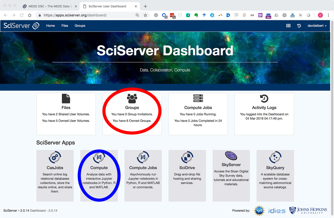
- Click login and create a new account. Once logged in you will be navigated with the following Dashboard page:

- Email pdc@jhu.edu to be added to the PARADIM user group and gain access to PARADIM specific resources.
You will receive a reply email within 24 hours inviting you to the PARADIM group. The next time you are login after being added to PARADIM group, your SciServer Dashboard will list the invitation in the “Groups” app (circled in red in the screenshot above). - Click “Groups” and accept the invitation.
- How to Create and Launch a Container
- Login to your SciServer account and start the Compute app (note that “Compute” and “Compute Jobs” are different and you need to open the “Compute”, circled in blue in the screenshot below)
- In Compute, use the green button to Create a computing container.
Be sure to:
a. type in a name for your container
b. select the “PARADIM” Compute Image from the drop-down menu
c. check the “PARADIM Data Collective” volume to add it to your container
In a few seconds you will return to the “Compute” screen and you can see your running container.
- Once your container is made, click the container to open a new browser tab accessing your compute container (If you are returning to a stopped container, you will have to click the green arrowhead to restart it).
The container mounts into a new browser tab showing the mounted volumes (paradim_data, storage, and temporary). The storage and temporary volumes are for your personal work. They will be available in any other SciServer container you make (they go with your account). The paradim_data storage is for data or work you want available to the whole PARADIM group.
Your storage volume is only 10 GB but is backed up and is permanent. Your temporary volume is part of 80 TB of storage shared between users. Temporary storage has no guarantee of long-term storage but can be used for weeks or even months at a time. You will be warned before it is cleaned up and given time to move anything you have stored there. The paradim_data volume is about 300 TB storage for sharing materials data. This is where experiment results will be shared.
- How to Open a Notebook
- You can now make a notebook. To make a new notebook use the “New” menu on the right-hand side of the browser as shown here:
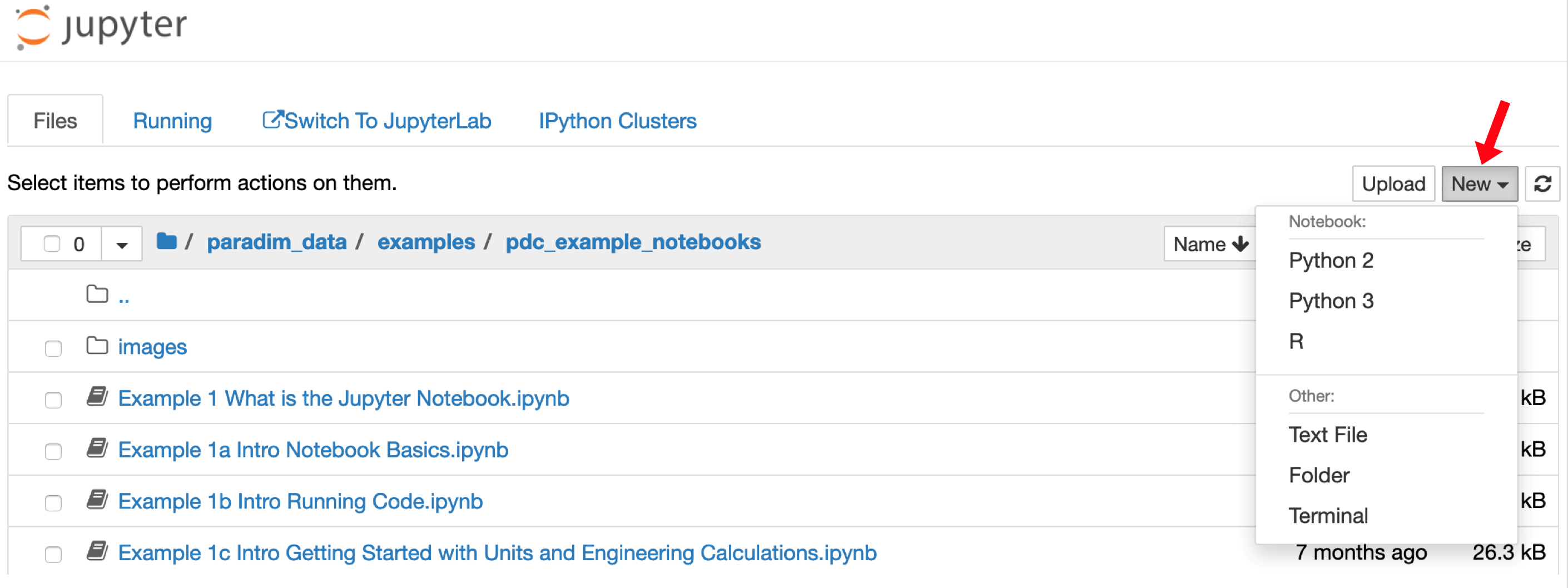
- Choose “Python 3” and a new browser tab will open with a blank notebook.
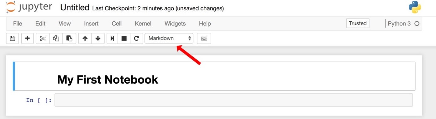
- In the first cell type “# My First Notebook” (without the quotes)
- Change the cell type to “markdown” and hit shift-enter.
Your notebook will look like this (the red arrow shows you the drop-down menu to make the cell "markdown" instead of code):
Notice that the kernel is Python 3 (shown on the right side) and that there are tools and menus you can look through and use. - Enter some Python code in the second cell and execute it.
Try 1+1 or try print ("All I dream about is reciprocal space.") - Save your notebook and continue following the tutorial to explore a range of SciServer notebook examples.
Please contact David Elbert (elbert@jhu.edu) or Nick Carey (ncarey4@jhu.edu) for any questions related to SciServer.
- Your First SciServer Tutorial
- Go back to the “Home” tab by clicking on the “Jupyter” logo, browse to the paradim_data volume and locate the “example>pdc_example_notebooks” folder. Open it.
- Open the “ReadMePlease.ipynb” notebook for basic information about the example notebooks. Everything in the examples directory is read-only. If you want your own copies of the notebooks to play with, follow the directions in ReadMePlease.ipynd to copy the example notebooks to your own, persistent storage. Explore the Jupyter window’s menu bars and tools. These include editing tools and the ability to change or restart the computational kernel.
- Close the notebook by using the File>Close and Halt in the Jupyter menubar.
- Open “Example 1a Intro Notebook Basics". This notebook is a general overview of using Jupyter. If you’re new to Jupyter, read through the notebook and follow examples to edit cells and make menu choices.
- Open “Example 1b Intro Running Code” to learn how to execute cells and run active code. Double-click your cursor into the first code cell (it has a gray background and the python code “a = 10”. Shift-enter to execute the cell. Execute the next cell (Shift-enter) to use the Python print statement to print back the value of a. Work through the other cells in Example 1b to get a feel for mixing execution and text in a notebook.
- Go back to the “Home” tab and go to the Jupyter tab labeled “Running.” There you will find what notebooks and terminals you have open and running. You can go back to them by clicking on them or you can shut them down here. N.B. if you shutdown a notebook from this tab you don’t know what was saved. This is a really useful tab to get back to something that you left running the last time you were on the Data Science Cloud (DSC).
- Example Notebook Tutorials Available on SciServer
Once you have followed the above steps successfully the system is now ready for you to explore some further notebook tutorials,
- Open the Example 5 notebook. Click in each cell to see the markdown (formatted text cells) and execute the calculations from top to bottom. There are four important things to learn in this notebook:
a. Jupyter has two modes: command and edit. Command mode is for moving around the notebook while edit mode lets you modify the contents of the cells. Esc puts you in command mode. Esc-enter puts you back in edit mode once you click into a cell.
b. You manually pick if a cell is code (executable) or markdown (formatted text). There is a drop-down menu to do (you can pick up key-stroke shortcuts later, but command mode M changes a cell to markdown and command mode Y changes it to code)
c. Cells need to be executed when you finish with your input. That means markdown (text) cells, too. Execute any cell with shift-enter.
d. You can use these notebooks to combine complex formatting, materials calculations, and something like a scanned image to fully investigate problems. - Open the Example 4 notebook. N.B. This notebook requires an updated key from the Materials Project. Go to https://www.materialsproject.org/ and login to the dashboard to get an API key. To use the Materials Project APIs, you need to get a new key every day.
a. Replace the API key in quotes of the first code cell in the Example 4 notebook with a fresh key.
b. Execute the cells in order to retrieve and display data from the Materials Project. The Materials Project is a data repository that has already calculated a range of properties for common materials. You can pull information directly into your notebooks to avoid duplicating that effort. - Open the Example 6 notebook. This notebook takes advantage of the preloaded Mantid environment in the MEDE-DSC. Mantid is a data analysis and visualization package created for neutron and muon scattering results from beamlines.
a. Read the text and execute the code in sequence. This notebook reads in a neutron data file from the ISIS Neutron Source Facility near Oxford.
b. Using Mantid calls, the cells plot the raw data as well as showing a smoothing function.
Mantid is the analysis package of choice at the Spallation Neutron Source (SNS) at Oak Ridge.
- Jupyter Keyboard Shortcuts
Frequently used:
Esc-goes to Command Mode where arrow keys let you navigate
Enter-goes to edit mode where you can type in cells
In Command Mode:
A-inserts new cell above
B-inserts new cell below
M-changes current cell to Markdown
Y-changes current cell to code
DD-(hit D twice) deletes the current cell
Shift-Tab- will show the Docstring for code object you just typed
?-Typing ? before a command and evaluating it will show the Docstring
Ctrl+Shift+hyphen will split the current cell into two at your cursor
Esc+F to find and replace in code
Esc+O to toggle cell output
Selecting Multiple Cells:
Shift-J or Shift-down- selects the next cell down
Shift-K or Shift-up selects the next cell above
Shift-M merges selected cells
You can delete/copy/cut/paste multiply selected cells
Multicursor support like Sublime. Click and drag mouse while holding down Alt.
- Additional Resources and References
- Graphing Tools
matplotlib is the de-facto standard. It’s activated with %matplotlib inline - Here’s a Dataquest Matplotlib Tutorial. Inline it can be a little slow because it is rendered on the server-side, but it’s easy and well known.
Seaborn is built over matplotlib and makes building more attractive plots easier. Just by importing Seaborn, your matplotlib plots are made ‘prettier’ without any code modification.
mpld3 provides an alternative renderer (using d3) for matplotlib code. Quite nice, though incomplete.
bokeh is a better option for building interactive plots.
plot.ly can generate nice plots - this used to be a paid service only but was recently open sourced.
Altair is a relatively new declarative visualization library for Python. It’s easy to use and makes great looking plots, however the ability to customize those plots is not nearly as powerful as in matplotlib. - Further Readings
Numerical Python: A Practical Techniques Approach for Industry, Robert Johansson, 2015, available online through JHU Libraries
Python: Pocket Primer, Oswald Campesato, 2012, available online through JHU Libraries
Data Wrangling with Python, Jacqueline Kazil and Katherine Jarmul,
Online Python Basics:
http://www.mantidproject.org/Introduction_To_Python (Exercises 1, 2,…)
http://cs231n.github.io/python-numpy-tutorial/
https://engineering.ucsb.edu/~shell/che210d/numpy.pdf